Text Analysis of Martha Ballard’s Diary (Part 2)
Given Martha Ballard’s profession as a midwife, it is no surprise that she carefully recorded the 814 births she attended between 1785 and 1812. These events were given precedence over more mundane occurrences by noting them in a separate column from the main entry. Doing so allowed her to keep track not only of the births, but also record payments and restitution for her work. These hundreds of births constituted one of the bedrocks of Ballard’s experience as a skilled and prolific midwife, and this is reflected in her diary.
As births were such a consistent and methodically recorded theme in Ballard’s life, I decided to begin my programming with a basic examination of the deliveries she attended. This examination would take the form of counting the number of deliveries throughout the course of the diary and grouping them by various time-related characteristics, namely: year, month, and day of the week.
Process and Results
The first basic step for performing a more detailed text analysis of Martha Ballard’s diary was to begin cleaning up the data. One step was to take all the words and (temporarily) turn every uppercase letter into a lowercase letter. This kept Python from seeing “Birth” and “birth” as two separate words. For the purposes of this particular program, it was more important to distill words into a basic unit rather than maintain the complexity of capitalized characters.
Once the data was scrubbed, we could turn to writing a program that would count the number of deliveries recorded in the diary. The program we wrote does the following:
- Checks to see if Ballard wrote anything in the “birth” column (the first column of the entries that she also used to keep track of deliveries)
- If she did write anything in that column, check to see if it contains any of the words: “birth”, “brt”, or “born”.
- I then printed the remainder of the entries that contained text in the “birth” column but did not contain one of the above words. From this short list I manually added an additional seven entries into the program, in which she appeared to have attended a delivery but did not record it using the above words.
Using these parameters, the program could iterate through the text and recognize the occurrence of a delivery. Now we could begin to organize these births.
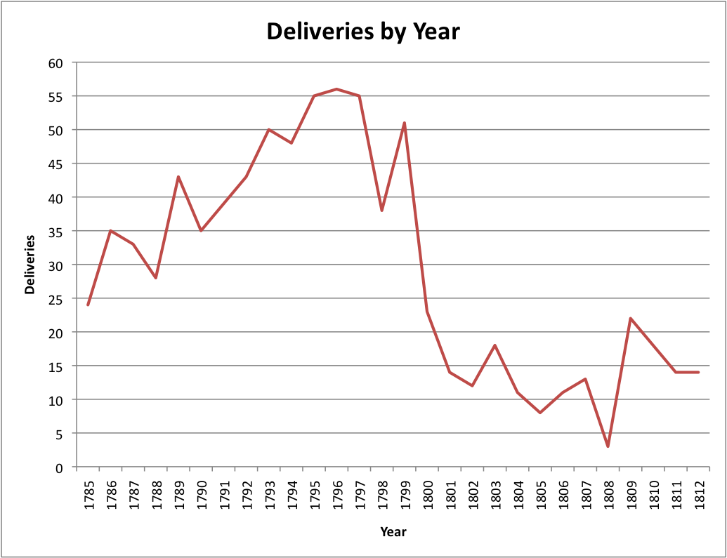
First, we returned the birth counts for each year of the diary, which were then inserted into a table and charted in Excel:
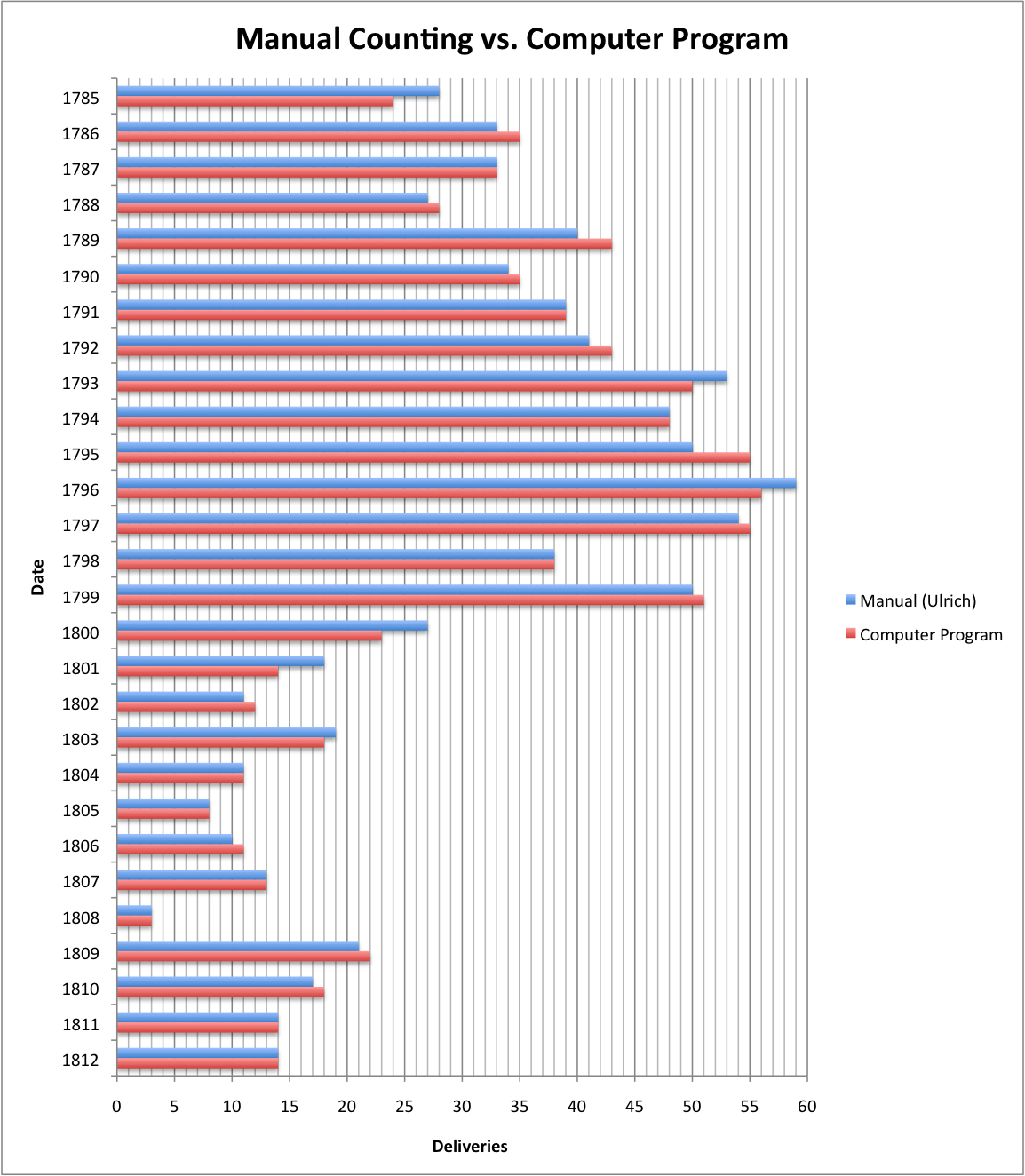
At the risk of turning my analysis into a John Henry-esque woman vs. machine, I compared my figures to the chart that Laurel Ulrich created in A Midwife’s Tale that tallied the births Ballard attended (on page 232 of the soft-cover edition). The two charts follow the same broad pattern:
Note: I reverse-built her chart by creating a table from the printed chart, then making my own bar graph. Somewhere in the translation I seem to have misplaced one of the deliveries (Ulrich lists 814 total, whereas I keep counting 813 on her graph). Sorry!
However, a closer look reveals small discrepancies in the numbers for each individual year. I calculated each year’s discrepancy as follows, using Ulrich’s numbers as the “true” figures (she is the acting President of the AHA, after all) from which my own figures deviated, and found that the average deviation for a given year was 4.86%. Apologies for the poor formatting, I had trouble inserting tables into Wordpress:
| Year | Deliveries Count | Difference | Deviation (from Ulrich) | |
| Manual (Ulrich) | Computer Program | |||
| 1785 | 28 | 24 | 4 | 14.29% |
| 1786 | 33 | 35 | 2 | 6.06% |
| 1787 | 33 | 33 | 0 | 0.00% |
| 1788 | 27 | 28 | 1 | 3.70% |
| 1789 | 40 | 43 | 3 | 7.50% |
| 1790 | 34 | 35 | 1 | 2.94% |
| 1791 | 39 | 39 | 0 | 0.00% |
| 1792 | 41 | 43 | 2 | 4.88% |
| 1793 | 53 | 50 | 3 | 5.66% |
| 1794 | 48 | 48 | 0 | 0.00% |
| 1795 | 50 | 55 | 5 | 10.00% |
| 1796 | 59 | 56 | 3 | 5.08% |
| 1797 | 54 | 55 | 1 | 1.85% |
| 1798 | 38 | 38 | 0 | 0.00% |
| 1799 | 50 | 51 | 1 | 2.00% |
| 1800 | 27 | 23 | 4 | 14.81% |
| 1801 | 18 | 14 | 4 | 22.22% |
| 1802 | 11 | 12 | 1 | 9.09% |
| 1803 | 19 | 18 | 1 | 5.26% |
| 1804 | 11 | 11 | 0 | 0.00% |
| 1805 | 8 | 8 | 0 | 0.00% |
| 1806 | 10 | 11 | 1 | 10.00% |
| 1807 | 13 | 13 | 0 | 0.00% |
| 1808 | 3 | 3 | 0 | 0.00% |
| 1809 | 21 | 22 | 1 | 4.76% |
| 1810 | 17 | 18 | 1 | 5.88% |
| 1811 | 14 | 14 | 0 | 0.00% |
| 1812 | 14 | 14 | 0 | 0.00% |
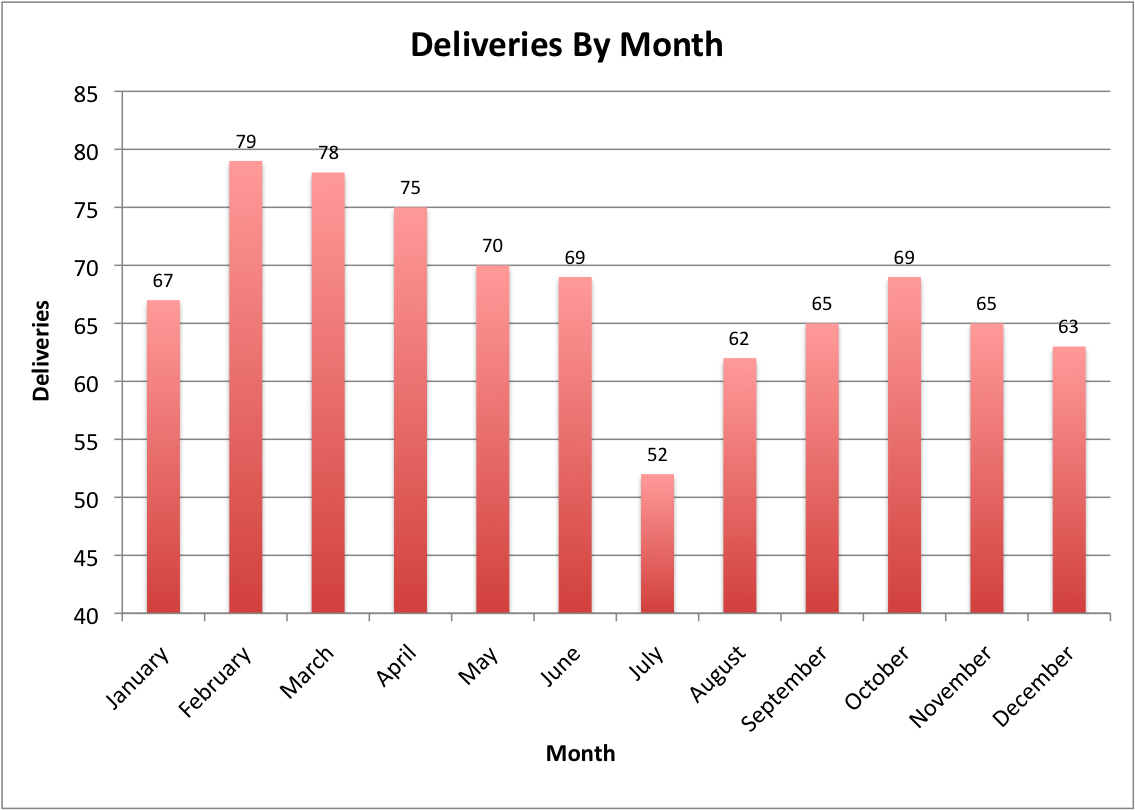
Keeping the knowledge in the back of my mind that my birth analysis differed slightly from Ulrich’s, I went on to compare my figures with other factors, including the frequency of deliveries by month over the course of the diary.
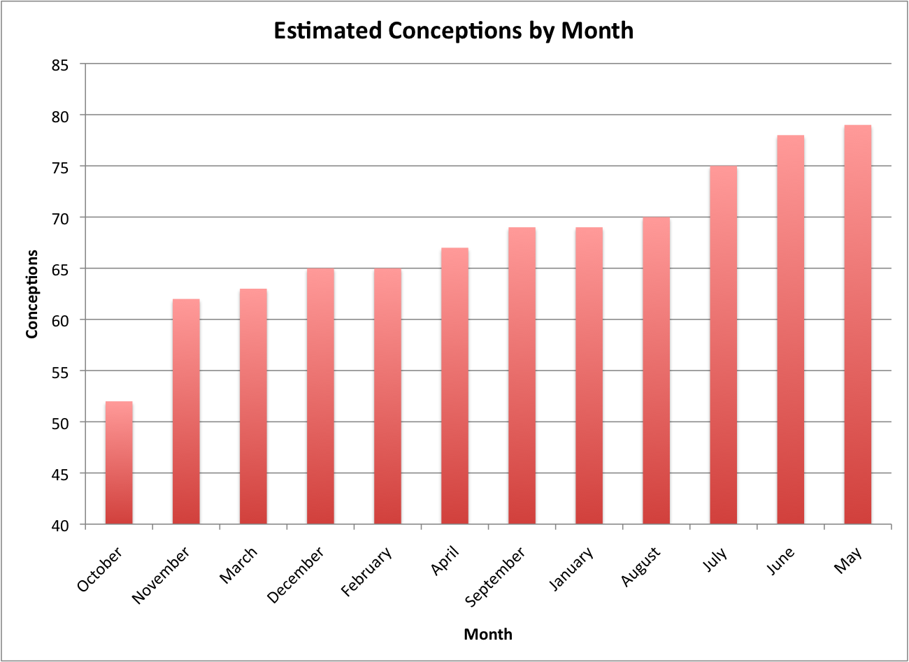
If we extend the results of this chart and assume a standard nine-month pregnancy, we can also determine roughly which months that Ballard’s neighbors were most likely to be having sex. Unsurprisingly, the warmer period between May and August appears to be a particularly fertile time:
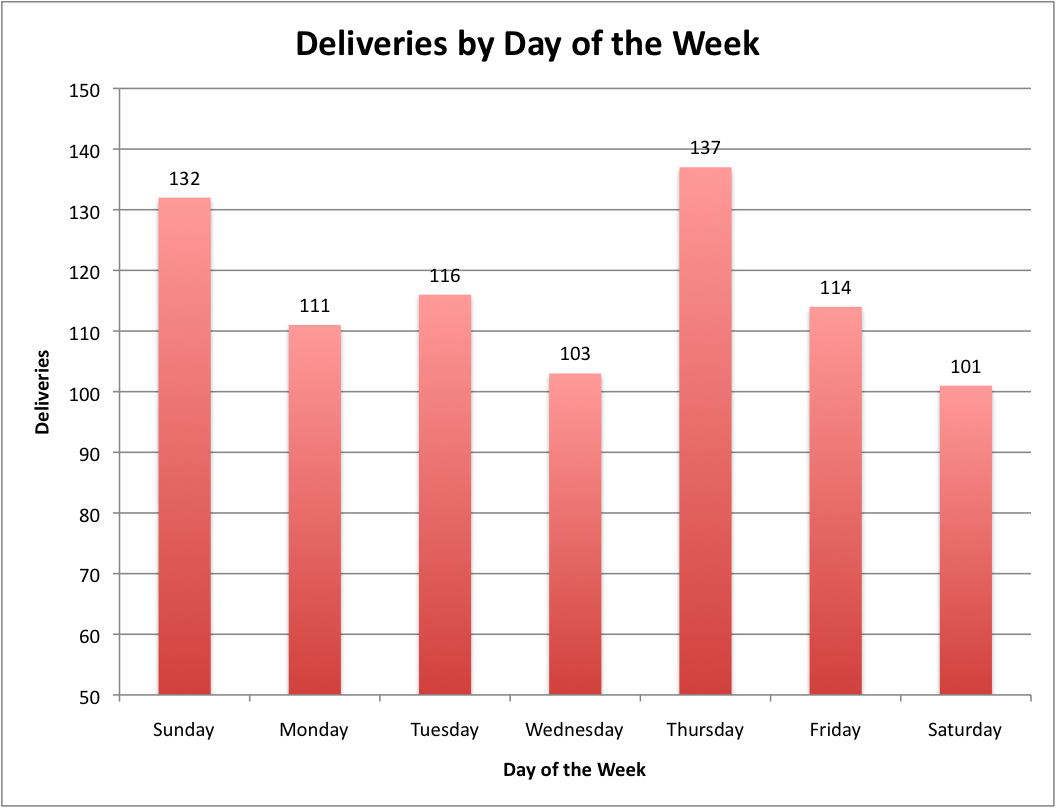
Finally, I looked at how often births occurred on different days of the week. There wasn’t a strong pattern, beyond the fact that Sunday and Thursday seemed to be abnormally common days for deliveries. I’m not sure why that was the case, but would love to hear speculation from any readers.
Analysis
The discrepancies between the program’s tally of deliveries and Ulrich’s delivery count speak to broader issues in “digital” text mining versus “manual” text mining:
Data Quality
Ulrich’s analysis is a result of countless hours spent eye-to-page with the original text. And as every history teacher drills into their students when conducting research, looking directly at the primary documents minimizes the degrees of interpretation that can alter the original documents. In comparison, my analysis is the result of the original text going through several levels of transformation, like a game of telephone:
Original text -> Typed transcription -> HTML tables -> Python list -> Text file -> Excel table/chart
Each level increases the chance of a mistake. For instance, a quick manual examination using the online version of the diary for 1785 finds an instance of a delivery (marked by ‘Birth’) showing up in the online HTML, but which does not appear in the “raw” HTML files our program is processing and analyzing.
On the other hand, a machine doesn’t get tired and miscount a word tally or accidently skip an entry.
Context
Ulrich brings to bear on the her textual analysis years of historical training and experience along with a deeply intimate understanding of Ballard’s diary. This allows her to take into account one of the most important aspects of reading a document: context. Meanwhile, our program’s ability to understand context is limited quite specifically to the criteria we use to build it. If Ballard attended a delivery but did not mark it in the standard “birth” column like the others, she might mention it more subtly in the main body of the entry. Whereas Ulrich could recognize this and count it as a delivery, our program cannot (at least with the current criteria).
Where the “traditional” skills of a historian come into play with data mining is in the arena of defining these criteria. Using her understanding of the text on a traditional level, Ulrich could create far, far superior criteria than I could for counting the number of deliveries Martha Ballard attends. The trick comes in translating a historian’s instinctual eye into a carefully spelled-out list of criteria for the program.
Revision
One area that is advantageous for digital text mining is that of revising the program. Hypothetically, if I realized at a later point that Ballard was also tallying births using another method (maybe a different abbreviated word), it’s fairly simple to add this to the program’s criteria, hit the “Run” button, and immediately see the updated figures for the number of deliveries. In contrast, it would be much, much more difficult to do so manually, especially if the realization came at, say, entry number 7,819. The prospect of re-skimming thousands of entries to update your totals would be fairly daunting.
